Hello everyone, probably everyone who works in an office or accounting is too familiar with Excel, right? But to fully utilize its features, especially creating spreadsheets efficiently, not everyone is adept at. Sometimes, manually drawing borders around cells is acceptable, but using Excel’s native Table feature is much more powerful. In this post, I’ll share some quick and easy ways to create tables in Excel, applicable for Excel 2010, 2013, 2016.
So, what makes an Excel (Excel Table) different from just manually drawing borders around cells? Fundamentally, it’s much smarter. Data within a Table is managed separately, tidily, and comes with many features:
- Add/delete rows and columns easily, with automatic expansion of the table.
- Built-in powerful filters right on the header, allowing sorting and filtering data.
- Formulas work better, with the ability to reference by column name instead of cumbersome cell addresses.
- Quickly change colors and table formats with predefined styles, looking professional instantly.
- Easy to create charts or PivotTables from table data.
In summary, creating a table using Excel’s Table feature significantly enhances data management and analysis compared to just drawing borders around cells, guys.
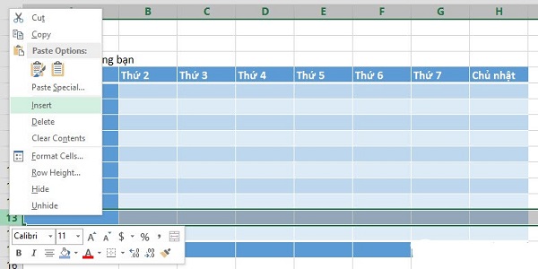 Professional formatted Excel worksheet using Table feature
Detailed Guide on How to Create Tables in Excel
Alright, now let’s get to the main part. There are 3 most common ways to create a table in Excel, choose based on your needs.
1. Using the Border Tool
This method is very basic; it’s not truly creating a Table as per Excel’s definition, but just drawing borders around data cells. If you just need a visual table without any smart features, this quick method is suitable.
Excel naturally works with grids of cells, so you can just select your data range, go to the Home tab, look for the dotted square icon (Border), click the small arrow next to it, and choose All Borders. That’s it—instant table with borders. Simple, quick, but only looks good — it’s not as “smart” as the other methods.
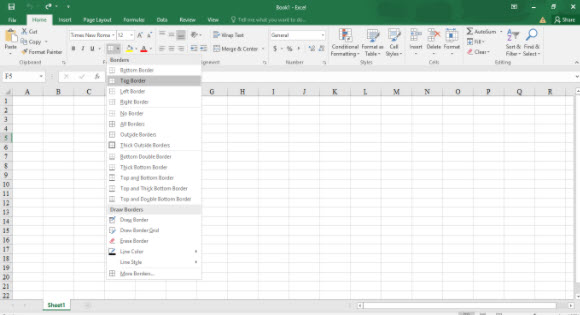 Using Border tool to quickly add borders to data range in Excel
2. Using Insert Table feature
This method creates a proper Excel Table. It converts your data range into an actual table object with full features.
- Step 1: Select your data range (including headers if available). Or simply click any cell within your data; Excel usually detects the range accurately. Then, go to the
Inserttab, and clickTable. Or quickly pressCtrl + T.
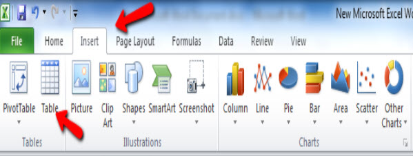 Choose Insert and then Table on Excel toolbar to create a data table
- Step 2: The
Create Tabledialog pops up. It shows the detected data range. Verify or select the correct range. Make sure the “My table has headers” box is checked if your data includes headers. If not, leave it unchecked, and Excel will generate default headers likeColumn 1,Column 2, etc., which you can rename later. Then clickOK.
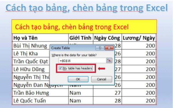 Create Table dialog in Excel confirming data range and headers
Done! Your data range is now a fancy table with alternating row colors and filter buttons on headers.
3. Quick Formatting as Table
This method also creates an Excel Table, similar to Insert Table, but allows you to choose the style (colors, fonts, borders, etc.) right from the start. Perfect for those who want a beautiful, professional-looking table without much customization.
- Step 1: Select your data range. Then go to the
Hometab, find theStylesgroup, and chooseFormat as Table.
 Access Format as Table from Home tab to pick a style
- Step 2: A list of Table Styles appears. Pick one that suits your taste. Then, the
Create Tabledialog appears again. Verify range, adjust header options, and clickOK.
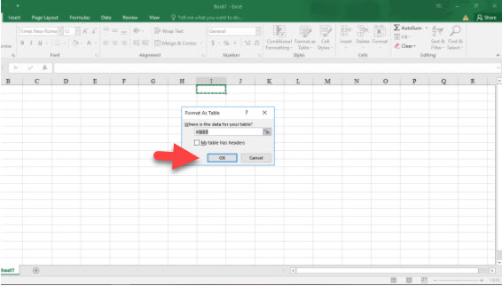 Confirm data range and headers after choosing style
Done! Your table now looks both smart and attractive, matching your chosen style.
How to delete or remove table formatting in Excel
Sometimes, after creating a table, you might want to revert back to normal cells. How to do that? It’s easy.
1. Convert to Range
This removes the Table features (like automatic expansion, filters, etc.), reverting it to a normal data range. Data and formatting (colors, fonts, borders) are retained.
- Step 1: Click any cell in the table. The
Table Designtab (orDesignin older versions) appears on the ribbon. Click it, find theToolsgroup, and clickConvert to Range.
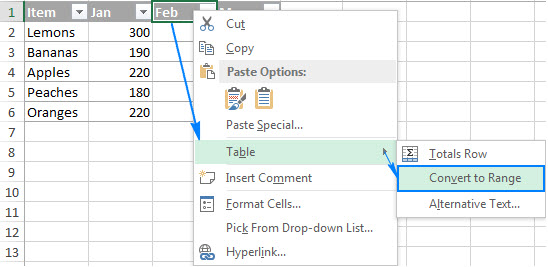 Use Convert to Range option in Table Design tab
- Step 2: Confirm in the dialog box, click
Yes.
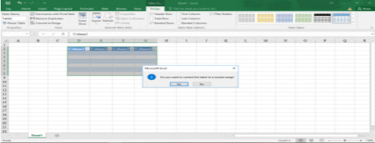 Confirm convert table to range dialog
Now your table is just plain cells, losing all Table features.
2. Clear table formatting
If you just want to remove the style of the table (colors, borders) but keep it as a Table with smart features, do this:
- Step 1: Click any cell in the table.
- Step 2: Go to
Table Design(orDesign), in theTable Stylesgroup, click theMorearrow (downward arrow with a hat) to expand styles. SelectClearat the bottom. Alternatively, choose theNonestyle (usually the first style in the group).
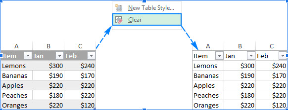 Choose Clear in Table Styles to remove default table styling
Note: This only removes styling applied by Table Styles. If you’ve manually added formats (like coloring individual cells), they won’t be removed. To clear all formats, select the range, go to Home, click Clear -> Clear Formats.
Conclusion
That’s all about the ways to create and delete tables in Excel I shared earlier. Overall, using Excel’s Table feature offers much more benefits than just manually drawing borders — it helps you manage data neatly, and makes calculation and analysis easier. Hope these tips help you work with Excel more efficiently and professionally. If you find this helpful, visit Softbuzz regularly for more tech tips and useful software knowledge!


