Microsoft Excel is the perfect spreadsheet tool for today’s office workers. So how to lock rows in excel as well as performing other simple operations with rows and columns. Read the following article for detailed and specific instructions!
How to lock rows in Excel 2010
Locking rows in Excel greatly helps in tracking statistical data sheets and calculations when there are too many columns. Scrolling up and down to view column properties can waste a lot of your time. Therefore, the method of locking rows in Excel will quickly solve this problem.
Don’t miss the standard Office installation available Microsoft Office 2010.
How to lock the header in Excel (lock one row)
To perform the method of locking rows in Excel, just:
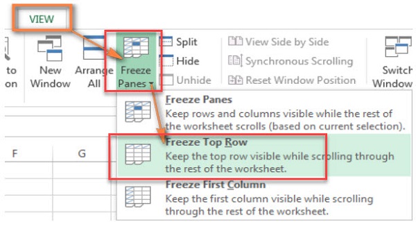
Highlight the header row and select the View tab -> select Freeze Panes -> choose Freeze Top Row. With just a few simple clicks on the toolbar, you can quickly lock the first row of the sheet.

Note: If you create a table with Excel Table, there’s no need for the additional step of locking rows. Because the header row of the table is always fixed at the top.
If you don’t know how to create a table, don’t miss this article.
Lock multiple rows in Excel
Depending on the purpose of your spreadsheet, you may need to lock different rows. Just follow these two simple steps:
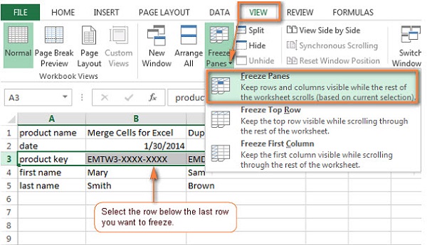
- Step 1: Select the row in the table you want to lock. For example, to lock the first two rows, select row A3 (or a specific cell in row A).

- Step 2: Choose View -> click the downward arrow icon in the Freeze Panes group -> select Freeze Panes.
The process of locking rows in various Excel versions is quite similar, with a slight difference in Excel 2003. In Excel 2003: click the Window icon on the toolbar -> choose Freezer Panes.
For other versions, the method of locking rows in Excel 2010 is exactly the same as in versions 2013 and 2016. So you can confidently perform the steps.
How to lock columns in Excel 2010
Similar to locking rows, you can also lock columns using the following methods:
Lock the first column in Excel
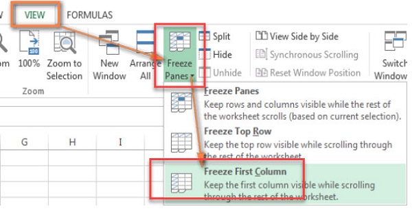
After selecting the column to lock, click on the View tab -> choose Freeze Panes -> select Freeze First Column.

Lock multiple columns in Excel
This operation is also very simple using the View tab. However, note that the column you want to lock must always start from column A and be on the top row. You cannot lock a column in the middle of the sheet.
After highlighting the column to be locked, choose View -> select Freeze Panes -> then select Freeze panes.
Lock a sheet area in Excel
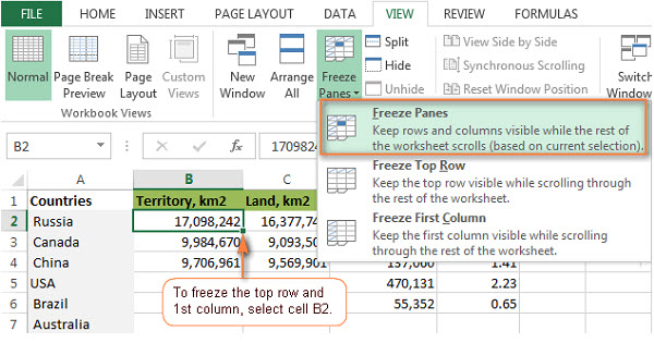
To lock a specific area including rows and columns, do as follows: highlight the area containing both rows and columns. Select the View tab, then choose Freeze Panes as described above.

Remove locking in Excel sheets
To remove the locking of rows, columns, or a sheet area in Excel, you need to use the View tab. The operation: highlight the locked rows, columns, or area -> select View -> pick Unfreeze Panes.
Besides locking operations, Excel also supports other pane-related actions such as:
- Hide rows, columns.
- Insert or delete sheets.
- Rename sheets.
Conclusion
Hopefully, with these instructions on how to lock rows in Excel, you can easily work with your sheets and create the spreadsheet as desired. For more updated information on software and computer tricks, click on our website: https://softbuzz.net/ – a beneficial info page for readers interested in technology!


